广度优先搜索（BFS，Breadth-First Search）

在战棋类游戏中（如高级战争），地图一般会被划分为网格，可移动单位一般都有一个移动步数范围，在玩家操控时会在地图上显示可移动范围，如下图中的红色坦克。要实现这一功能就可使用BFS算法了。

基本概念

算法从起始节点出发，首先访问与起始节点距离为 1 的所有节点，然后访问距离为 2 的所有节点，依此类推。在 BFS 中，所有边的权重相同，因此每次移动到相邻节点的代价相等（无权图）。

算法步骤

BFS 使用队列（Queue）数据结构来实现。

初始化：
- 将起始节点标记为已访问，并将其加入队列。
- 创建一个记录节点是否被访问的布尔数组或集合。
开始遍历：
- 从队列中取出一个节点，访问该节点。
- 将该节点的所有未访问过的邻接节点标记为已访问，并依次加入队列。
继续遍历：
- 重复上述步骤，直到队列为空或找到目标节点。

算法实现

以下是 BFS 算法的伪代码和 Python 实现：

伪代码

BFS(graph, start):
    create a queue Q
    create a set of visited nodes
    enqueue start to Q
    add start to visited

    while Q is not empty:
        node = dequeue from Q
        for each neighbor in graph.neighbors(node):
            if neighbor is not in visited:
                enqueue neighbor to Q
                add neighbor to visited

Python 实现

from collections import deque

def bfs(graph, start):
    # 初始化队列和已访问集合
    queue = deque([start])
    visited = set([start])

    while queue:
        node = queue.popleft()
        print(node)  # 访问节点

        for neighbor in graph[node]:
            if neighbor not in visited:
                visited.add(neighbor)
                queue.append(neighbor)

示例

假设有一个简单的无权图如下：

A - B - C
|   |
D - E

调用bfs(graph, 'A')，遍历顺序为：A -> B -> D -> C -> E。

总结

BFS 是一种简单的图遍历算法，特别适用于无权图的最短路径查找和层级遍历。但是在寻路算法中，其无目的性使其多了很多不必要的计算。

Best First Search

基于广度优先搜索，引入了启发式搜索。

在 Best First Search 中，不会对所有的相邻路径进行搜索，而是基于一个优先度来搜索。此优先度一般使用曼哈顿距离来计算。

即给定目标点，待搜索路径点会计算一个和目标点的曼哈顿距离，距离越短优先度越高。

相比较广度优先搜索，有目的性搜索减少了很多不必要的计算。

但是 Best First Search 找出的路径不一定是最优解。

A*

A*（A-star）算法是一种用于图搜索的启发式算法，广泛应用于路径寻找和图遍历。它结合了 Dijkstra 算法的最短路径搜索和启发式方法的预判能力，既能确保找到最优路径，又在大多数情况下高效运行。

1. 基本概念

启发式搜索：使用启发式函数估计当前节点到目标节点的代价，从而指导搜索方向。
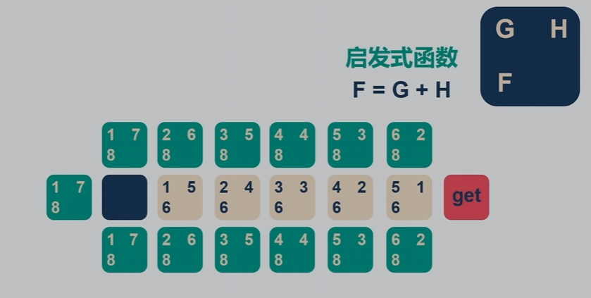
评估函数：A*算法使用评估函数(f(n) = g(n) + h(n))，其中：
- (g(n))：从起点到当前节点 n 的实际代价。有时可以通过 g(n-1)计算得来。
- (h(n))：从当前节点 n 到目标节点的估计代价（启发式函数）。

2. 算法步骤

A*算法使用优先队列（Priority Queue）来实现，其步骤如下：

初始化：
- 将起始节点放入开放列表（Open List），初始的(g(n) = 0)。
- 关闭列表（Closed List）用于存储已访问节点。
迭代过程：
- 从开放列表中取出具有最低(f(n))值的节点作为当前节点。
- 如果当前节点是目标节点，则结束搜索，构建路径。
- 否则，将当前节点移至关闭列表。
- 对当前节点的每个相邻节点：
  - 如果相邻节点在关闭列表中，则忽略。
  - 计算相邻节点的(g)值，如果该节点不在开放列表中或新的(g)值更小，则更新相邻节点的(g)和(f)值，并将其父节点设置为当前节点。
  - 如果相邻节点不在开放列表中，则将其添加进去。

3. 算法实现

以下是 A*算法的伪代码和 Python 实现：

伪代码

A*(start, goal):
    openList = priority queue containing start
    closedList = empty set

    g(start) = 0
    f(start) = g(start) + h(start)

    while openList is not empty:
        current = node in openList with lowest f(node)
        if current is goal:
            return reconstruct_path(goal)

        remove current from openList
        add current to closedList

        for each neighbor of current:
            if neighbor in closedList:
                continue

            tentative_g = g(current) + d(current, neighbor)

            if neighbor not in openList:
                add neighbor to openList
            elif tentative_g >= g(neighbor):
                continue

            set parent of neighbor to current
            g(neighbor) = tentative_g
            f(neighbor) = g(neighbor) + h(neighbor)

    return failure

Python 实现

import heapq

def a_star(graph, start, goal, h):
    open_list = []
    heapq.heappush(open_list, (0, start))
    came_from = {}
    g_score = {start: 0}
    f_score = {start: h(start)}

    while open_list:
        _, current = heapq.heappop(open_list)

        if current == goal:
            return reconstruct_path(came_from, start, goal)

        for neighbor, cost in graph[current]:
            tentative_g_score = g_score[current] + cost
            if neighbor not in g_score or tentative_g_score < g_score[neighbor]:
                came_from[neighbor] = current
                g_score[neighbor] = tentative_g_score
                f_score[neighbor] = tentative_g_score + h(neighbor)
                heapq.heappush(open_list, (f_score[neighbor], neighbor))

    return None

def reconstruct_path(came_from, start, goal):
    path = [goal]
    while path[-1] != start:
        path.append(came_from[path[-1]])
    path.reverse()
    return path

4. 启发式函数

启发式函数 (h(n)) 是 A*算法的关键，其选择会影响算法的效率和正确性。常用的启发式函数有：

曼哈顿距离：适用于网格图，每次移动的代价相等。
欧几里得距离：适用于实际距离作为代价的图。
切比雪夫距离：适用于允许对角移动的网格图。

5. 应用场景

A*算法广泛应用于需要路径规划的领域，包括：

游戏开发：NPC 路径规划、迷宫求解。
机器人导航：移动机器人路径规划。
地图服务：GPS 导航、地图应用中的路线规划。

总结

A*算法是一个功能强大且灵活的路径寻找算法，通过结合实际代价和启发式估计，可以高效地找到从起点到目标点的最优路径。在实际应用中，选择合适的启发式函数是确保算法效率和准确性的关键。

Theta*

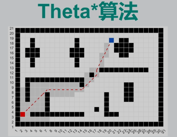
Theta*算法是 A*算法的扩展版本，它在路径规划中提供了一种改进（加入了射线探测），能够生成更短、更自然的路径，特别是对于网格图。Theta*算法的主要特点是允许对角线和直线穿越多个网格单元，而不仅仅是移动到相邻的单元，从而避免了 A*中常见的“锯齿状”路径。此时一般使用欧式距离。

1. 基本概念

线性插值：Theta*通过线性插值判断两点之间的直线是否可行，从而减少路径中的拐点。
亲节点（Parent Node）：每个节点不仅记录从哪个节点访问到它，还记录访问该节点时的起始节点，这样可以跳过中间节点进行直接连接。

2. 算法步骤

Theta*算法在 A*算法的基础上进行修改，其步骤如下：

初始化：
- 将起始节点放入开放列表（Open List），并将其父节点设为自身。
- 创建记录各节点的父节点（Parent）和(g)值的数组。
迭代过程：
- 从开放列表中取出具有最低(f(n))值的节点作为当前节点。
- 如果当前节点是目标节点，则结束搜索，构建路径。
- 否则，将当前节点移至关闭列表。
- 对当前节点的每个相邻节点：
  - 如果相邻节点在关闭列表中，则忽略。
  - 计算从当前节点的父节点直接到相邻节点的代价（即直线距离），如果比从当前节点再到相邻节点的代价小，则更新相邻节点的父节点为当前节点的父节点，否则更新为当前节点。（和 A*算法的主要区别，如下图所示，🟦 为当前节点，🔵 为父节点，🔺 为相邻节点。可以看到上下两个相邻节点可以直接和父节点相连（$cost = \sqrt{2}$），而无需经由当前节点（$cost=2$））
  - 更新相邻节点的(g)值和(f)值，如果相邻节点不在开放列表中，则将其添加进去。

3. 算法实现

以下是 Theta*算法的伪代码和 Python 实现：

伪代码

Theta*(start, goal):
    openList = priority queue containing start
    closedList = empty set
    parent[start] = start
    g(start) = 0
    f(start) = g(start) + h(start)

    while openList is not empty:
        current = node in openList with lowest f(node)
        if current is goal:
            return reconstruct_path(parent, start, goal)

        remove current from openList
        add current to closedList

        for each neighbor of current:
            if neighbor in closedList:
                continue

            if line_of_sight(parent[current], neighbor):
                tentative_g = g(parent[current]) + distance(parent[current], neighbor)
                if tentative_g < g(neighbor):
                    parent[neighbor] = parent[current]
                    g(neighbor) = tentative_g
                    f(neighbor) = g(neighbor) + h(neighbor)
                    if neighbor not in openList:
                        add neighbor to openList
            else:
                tentative_g = g(current) + distance(current, neighbor)
                if tentative_g < g(neighbor):
                    parent[neighbor] = current
                    g(neighbor) = tentative_g
                    f(neighbor) = g(neighbor) + h(neighbor)
                    if neighbor not in openList:
                        add neighbor to openList

    return failure

Python 实现

import heapq
import math

def line_of_sight(grid, start, end):
    # 实现线性插值检查两点之间的直线是否可通
    x0, y0 = start
    x1, y1 = end
    dx, dy = x1 - x0, y1 - y0
    steps = max(abs(dx), abs(dy))
    for i in range(steps + 1):
        x = int(x0 + i * dx / steps)
        y = int(y0 + i * dy / steps)
        if grid[y][x] == 1:  # 假设1代表障碍物
            return False
    return True

def theta_star(grid, start, goal, h):
    open_list = []
    heapq.heappush(open_list, (0, start))
    parent = {start: start}
    g_score = {start: 0}
    f_score = {start: h(start)}

    while open_list:
        _, current = heapq.heappop(open_list)

        if current == goal:
            return reconstruct_path(parent, start, goal)

        for neighbor in get_neighbors(grid, current):
            if line_of_sight(grid, parent[current], neighbor):
                tentative_g_score = g_score[parent[current]] + distance(parent[current], neighbor)
                if neighbor not in g_score or tentative_g_score < g_score[neighbor]:
                    parent[neighbor] = parent[current]
                    g_score[neighbor] = tentative_g_score
                    f_score[neighbor] = tentative_g_score + h(neighbor)
                    heapq.heappush(open_list, (f_score[neighbor], neighbor))
            else:
                tentative_g_score = g_score[current] + distance(current, neighbor)
                if neighbor not in g_score or tentative_g_score < g_score[neighbor]:
                    parent[neighbor] = current
                    g_score[neighbor] = tentative_g_score
                    f_score[neighbor] = tentative_g_score + h(neighbor)
                    heapq.heappush(open_list, (f_score[neighbor], neighbor))

    return None

def distance(point1, point2):
    return math.hypot(point2[0] - point1[0], point2[1] - point1[1])

def reconstruct_path(parent, start, goal):
    path = [goal]
    while path[-1] != start:
        path.append(parent[path[-1]])
    path.reverse()
    return path

def get_neighbors(grid, node):
    neighbors = []
    x, y = node
    for dx in [-1, 0, 1]:
        for dy in [-1, 0, 1]:
            if dx == 0 and dy == 0:
                continue
            nx, ny = x + dx, y + dy
            if 0 <= nx < len(grid[0]) and 0 <= ny < len(grid):
                neighbors.append((nx, ny))
    return neighbors

4. 应用场景

Theta*算法适用于需要生成更直、更自然路径的场景，如：

机器人导航：移动机器人路径规划，减少转弯，提高路径效率。
游戏开发：生成自然的 NPC 路径，避免锯齿状路径。
地图服务：复杂地形中的路径规划，如无人机导航。

总结

Theta*算法通过允许节点之间的直接连接，提高了路径的平滑性和自然性。它在实际应用中特别适用于需要生成直线路径或减少转弯的场景，如机器人导航和游戏开发。在这些领域，Theta*提供了一种更优的路径规划方案。

跳点搜索算法

跳点搜索（Jump Point Search，JPS）是一种优化的路径搜索算法，专门设计用于加速 A算法在网格图上的运行。JPS 通过跳过冗余节点，减少了 A算法的搜索空间，从而提高了效率。

1. 基本概念

跳点（Jump Point）：是路径上的关键点，这些点决定了路径的转折点或方向改变点。
强制邻居（Forced Neighbor）：在搜索过程中必须考虑的邻居节点，以确保不会遗漏潜在的最短路径。（在碰撞体四周）

2. 算法步骤

JPS 通过以下步骤进行优化：

初始化：
- 与 A*算法类似，初始化起始节点的开放列表、关闭列表以及相应的代价值。
跳跃过程：
- 从当前节点沿一个方向“跳跃”，直到遇到以下情况之一：
  - 到达目标节点。
  - 遇到障碍物。
  - 找到一个跳点（转折点或强制邻居）。
跳点的确定：
- 使用启发式方法判断当前方向上的强制邻居，确定跳点。
- 强制邻居是在当前方向上必须检查的节点，确保路径不会遗漏。
路径记录：
- 记录路径上的跳点，并将这些跳点加入开放列表。

如下图：蓝色和绿色点为跳点，蓝色为已访问的跳点

3. 算法实现

以下是 JPS 算法的伪代码和 Python 实现：

伪代码

JPS(start, goal):
    openList = priority queue containing start
    closedList = empty set
    g(start) = 0
    f(start) = g(start) + h(start)

    while openList is not empty:
        current = node in openList with lowest f(node)
        if current is goal:
            return reconstruct_path(current)

        remove current from openList
        add current to closedList

        for each direction in possible_directions:
            neighbor = jump(current, direction, goal)
            if neighbor is not None:
                if neighbor in closedList:
                    continue
                tentative_g = g(current) + distance(current, neighbor)
                if neighbor not in openList or tentative_g < g(neighbor):
                    parent[neighbor] = current
                    g(neighbor) = tentative_g
                    f(neighbor) = g(neighbor) + h(neighbor)
                    if neighbor not in openList:
                        add neighbor to openList

    return failure

jump(current, direction, goal):
    next = current + direction
    if next is blocked or out of bounds:
        return None
    if next == goal:
        return next
    if has_forced_neighbors(next, direction):
        return next
    return jump(next, direction, goal)

Python 实现

import heapq
import math

def jps(grid, start, goal, h):
    open_list = []
    heapq.heappush(open_list, (0, start))
    g_score = {start: 0}
    parent = {start: None}

    while open_list:
        _, current = heapq.heappop(open_list)

        if current == goal:
            return reconstruct_path(parent, start, goal)

        for direction in get_directions():
            neighbor = jump(grid, current, direction, goal, parent, g_score)
            if neighbor:
                tentative_g = g_score[current] + distance(current, neighbor)
                if neighbor not in g_score or tentative_g < g_score[neighbor]:
                    g_score[neighbor] = tentative_g
                    f_score = tentative_g + h(neighbor)
                    heapq.heappush(open_list, (f_score, neighbor))
                    parent[neighbor] = current

    return None

def jump(grid, current, direction, goal, parent, g_score):
    x, y = current
    dx, dy = direction
    next_node = (x + dx, y + dy)

    # 障碍物或者边界
    if not in_bounds(grid, next_node) or grid[next_node[1]][next_node[0]] == 1:
        return None
    # 终点
    if next_node == goal:
        return next_node
    # 是否有强制邻居
    if has_forced_neighbors(grid, next_node, direction):
        return next_node
    # 斜方向
    if dx != 0 and dy != 0:
        # 分解成水平和垂直分量搜索
        # 如果这两个搜索方向上有终点或者强制邻居，则返回这一节点
        # 表示此节点是一个跳点
        if jump(grid, next_node, (dx, 0), goal, parent, g_score) or jump(grid, next_node, (0, dy), goal, parent, g_score):
            return next_node
    # 继续沿着方向搜索
    return jump(grid, next_node, direction, goal, parent, g_score)

def get_directions():
    return [(-1, 0), (1, 0), (0, -1), (0, 1), (-1, -1), (-1, 1), (1, -1), (1, 1)]

def distance(node1, node2):
    return math.hypot(node2[0] - node1[0], node2[1] - node1[1])

def reconstruct_path(parent, start, goal):
    path = [goal]
    while path[-1] != start:
        path.append(parent[path[-1]])
    path.reverse()
    return path

def in_bounds(grid, node):
    x, y = node
    return 0 <= x < len(grid[0]) and 0 <= y < len(grid)

def has_forced_neighbors(grid, node, direction):
    x, y = node
    dx, dy = direction
    neighbors = [
        (x - dy, y + dx), (x + dy, y - dx),  # Orthogonal to direction
        (x - dx, y + dy), (x + dx, y - dy)   # Diagonal to direction
    ]
    for nx, ny in neighbors:
        if in_bounds(grid, (nx, ny)) and grid[ny][nx] == 0:
            return True
    return False

主流程分析：

这段代码实现了跳点搜索（Jump Point Search, JPS）算法中的主循环逻辑，结合 A*算法的启发式搜索来找到从起点到终点的最优路径。下面是逐行解析：

while open_list:
    _, current = heapq.heappop(open_list)

    if current == goal:
        return reconstruct_path(parent, start, goal)

    for direction in get_directions():
        neighbor = jump(grid, current, direction, goal, parent, g_score)
        if neighbor:
            tentative_g = g_score[current] + distance(current, neighbor)
            if neighbor not in g_score or tentative_g < g_score[neighbor]:
                g_score[neighbor] = tentative_g
                f_score = tentative_g + h(neighbor)
                heapq.heappush(open_list, (f_score, neighbor))
                parent[neighbor] = current

详细解释

主循环：
```
1
while open_list:
```
- 当open_list（优先队列）不为空时，持续执行循环。open_list保存待探索的节点。
从优先队列中取出当前节点：
```
1
_, current = heapq.heappop(open_list)
```
- 使用heapq.heappop从优先队列open_list中取出优先级最高的节点，即具有最低f_score的节点，存入current。_存储的是f_score，但这里并不需要使用它。

检查是否到达目标节点：

if current == goal:
    return reconstruct_path(parent, start, goal)

如果当前节点是目标节点，调用reconstruct_path函数重建路径，并返回结果。

获取所有可能的移动方向：
```
1
for direction in get_directions():
```
- 获取所有可能的移动方向（例如，上、下、左、右或对角线）。

跳点搜索：

neighbor = jump(grid, current, direction, goal, parent, g_score)

调用jump函数从当前节点沿指定方向进行跳跃，寻找下一个跳点。返回的neighbor是找到的下一个跳点或None。

处理找到的邻居节点：

if neighbor:
    tentative_g = g_score[current] + distance(current, neighbor)
    if neighbor not in g_score or tentative_g < g_score[neighbor]:
        g_score[neighbor] = tentative_g
        f_score = tentative_g + h(neighbor)
        heapq.heappush(open_list, (f_score, neighbor))
        parent[neighbor] = current

如果找到有效的邻居节点：
- 计算从起点到该邻居节点的临时距离（tentative_g）。
- 如果该邻居节点未被探索过，或找到了一条更短的路径到该邻居节点：
  - 更新邻居节点的g_score。
  - 计算邻居节点的f_score（f_score = g_score + h_score），其中h(neighbor)是从邻居节点到目标节点的启发式估计距离。
  - 将邻居节点及其f_score加入优先队列open_list。
  - 记录邻居节点的父节点为当前节点。

主要函数和数据结构

open_list: 优先队列，存储待探索的节点及其f_score。
heapq.heappop: 从优先队列中取出具有最低f_score的节点。
goal: 目标节点。
reconstruct_path: 重建从起点到目标节点的路径。
get_directions: 获取所有可能的移动方向。
jump: 执行跳点搜索，从当前节点沿指定方向跳跃，找到下一个跳点。
g_score: 字典，存储从起点到各节点的实际距离。
distance: 计算两个节点之间的实际距离。
h: 启发函数，估计从某节点到目标节点的距离。
heapq.heappush: 将节点及其f_score加入优先队列open_list。
parent: 字典，存储每个节点的父节点，用于路径重建。

4. 关键点解释

跳点：跳点是路径上的关键点，跳过了中间的冗余节点。
强制邻居：在判断跳点时，必须检查的邻居节点，以确保不会遗漏最短路径。
线性搜索：从当前节点沿一个方向进行线性搜索，直到找到跳点或遇到障碍。

5. 应用场景

JPS 特别适合用于以下场景：

游戏开发：在大规模网格地图中，快速生成最优路径。
机器人导航：在网格化环境中，规划高效路径。
地图服务：优化大规模网格地图上的路径查询。

6. 时间复杂度和空间复杂度

时间复杂度：在理想情况下，JPS 显著减少了节点的扩展数量，因此比 A更快，尤其在空旷区域。然而，最坏情况下，时间复杂度仍与 A相同，为 O(b^d)，其中 b 是分支因子，d 是路径深度。
空间复杂度：与 A*类似，为 O(b^d)，因为需要存储开放列表和关闭列表中的节点。

总结

跳点搜索通过跳过冗余节点，优化了 A*算法在网格图上的运行。它能够显著减少搜索空间，从而提高路径规划的效率，适用于需要高效路径搜索的各种应用场景。

注：以上部分内容通过 ChatGpt 生成

广度优先搜索（BFS，Breadth-First Search）

基本概念

算法步骤

算法实现

伪代码

Python 实现

示例

总结

Best First Search

A*

1. 基本概念

2. 算法步骤

3. 算法实现

伪代码

Python 实现

4. 启发式函数

5. 应用场景

总结

Theta*

1. 基本概念

2. 算法步骤

3. 算法实现

伪代码

Python 实现

4. 应用场景

总结

跳点搜索算法

1. 基本概念

2. 算法步骤

3. 算法实现

伪代码

Python 实现

主流程分析：

详细解释

主要函数和数据结构

4. 关键点解释

5. 应用场景

6. 时间复杂度和空间复杂度

总结

CATALOG

FEATURED TAGS